When you dig into the history of mapping, it’s remarkable how certain things come about. If you zoom in far enough, you discover seemingly coincidental occurrences that ended up playing pivotal roles in the development of digital maps and the product we now call “GIS.” It’s interesting to see how these connections mesh together when you zoom back out.
Take the database, for example: did Herman Hollerith (who we’ll talk about later in this article) think when he was sitting on a train in the late 1800s watching conductors punch holes in tickets that this would one day play a role in the development of the first database, which would eventually shape the field of GIS (Beninger 1997, 411-412)? Probably not. He was just a curious person being observant while sitting on the train. But it’s fascinating how these kinds of events are all over the timeline of the history of GIS.
Advancements in Mapping Techniques
To understand the development of GIS through all these coincidental events, let’s start back at the days of British colonization. The British had an early interest in mapping and navigation. “Why is that?” you might wonder. Well the British wanted to expand their resources, riches, and power, and having good maps could help them achieve this goal.
At this time in history, maps weren’t just symbols of power — they conferred power. As Simon Garfield argues in On the Map, with a good map, a military had an advantage in battle and a king knew how much land could be taxed. So it makes sense that the British had taken an interest in this field and had a desire to map their territories (Garfield 2013, 194).
The British took mapping to the next level in the mid to late 1700s with the British Ordnance Survey (Ordnance Survey “Our History” 2019) and The Great Trigonometrical Survey of India (a British colony at the time). This survey-based mapping marked a shift from a routing and descriptive-based process to a mathematical, grid-based technique using triangulation (Garfield 2013, 192). It also introduced the notion of fixed reference points (based on a datum) and scalability to the world of mapping.
The British Ordinance Survey (Winfields Outdoors Image 1 from “Interview With Ordnance Survey - History & Future of OS Maps”)

The Great Trigonometrical Survey India 1870 (Daniel Fernández Pascual Great Trigonometrical Survey of India 2012)

These advancements made it possible to create accurate cadastre, land, and natural resource maps and eventually paved the way for spatial analysis and map overlays, as accurate and scalable maps could be overlaid and analyzed for spatial patterns.
Spatial Analysis and Map Overlays
Without the availability of the Ordnance maps and the advancements made through Britain’s general obsession with mapping, the outbreak of cholera in a London neighborhood in 1854 could have done much more damage. But John Snow, a British physician, was able to use those maps and analyze the relationship between cholera deaths and water pumps in order to prove that the water was spreading the epidemic (GIS Geography “The Remarkable History of GIS” 2019). This was innovative in 1854, but, I would argue that place and heritage also played a role. If Snow hadn’t been in Britain during that time, and if Britain hadn’t had so many mapping developments, Snow may have taken a different — and possibly longer — path in solving the cholera outbreak.
John Snow Cholera Map 1854 (Micronautes Broad Street Map/Broadwick Street Water Pump 2017)

The Database
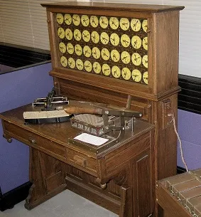
Now, enter the year 1887 as the USCB is still painfully tabulating the 1880 census. The Bureau knows that in two years the process will begin again — unless there is a more innovative method to speed it up. Herman Hollerith (sound familiar?) hears about their struggle and he recalls the train conductors. He remembers how they punched patterns on passenger tickets to capture information about the traveler. That memory sparks an idea in his mind that leads him to invent a tabulation machine (USCB “Herman Hollerith” 2018).
His device allowed the USCB to process and store the results on punch cards, ultimately saving tons of time. This tabulation machine eventually grew into the first database, which then became the precursor to the electronic computer. These inventions were driven by the need to speed up tabulation.
Hollerith’s Tabulation Machine (Adam Schuster Proto IBM 2007)
Hollerith’s Punch Card (Library of Congress Image of punched card of Herman Hollerith 1895)

Interestingly enough, Hollerith’s company was eventually merged into what we now know as IBM (which we’ll come back to later), and punch card technology played a critical role in computer programming and digital mapping well into the mid-1970s. Throughout that time, punch cards were how programmers created, edited, and stored their programs (Fisk 2005).
Canada Geographic Information System
Jump forward to the twentieth-century and, yet again, problem-solving that led another British-born scholar into exploring map overlays. This is exactly what was on the mind of geographer Roger Tomlinson in 1962 when he struck up a conversation with Lee Pratt (Tomlinson 2012). At the time, Tomlinson was working for an aerial surveying company in Canada, and Pratt was the newly appointed head of the Canadian Land Inventory. As chance would have it, they were seated next to each other on a flight, and they started chatting about natural resources and land management in Canada’s vast territory. For Tomlinson, the timing couldn’t have been more ideal.
In the years leading up to this encounter, Tomlinson had been working on a British aid project with the Kenyan government to locate suitable areas for tree cultivation in Kenya. The goal of the project was for Britain to assist Kenya (a former British colony) in creating its own paper. Locating suitable land for tree cultivation involved numerous map overlays. It was during this process that Tomlinson realized that digital maps would be better suited for this level of analysis, so he started exploring the idea of computers and digital mapping. But before Tomlinson could do anything with his ideas, the project ran out of money.
So as you can imagine, Tomlinson spared little detail when describing to Pratt how digital mapping could improve land management at the Canadian Land Inventory.
Ultimately, it was this chance encounter between Tomlinson and Pratt that eventually led to the creation of the Canadian Geographic Information System (CGIS) in the early 1960s, which is considered the first GIS (Poiker and Crain 2006). For Tomlinson, this partnership provided the right combination of money, interest, and feasibility, and because of Tomlinson’s early pioneering work at CGIS, he is generally recognized as the “father of GIS” (“Roger Tomlinson,” University Consortium for Geographic Information Science).
IBM
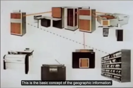
The development of CGIS was also when IBM entered the GIS picture: in the mid 1960s IBM was hired to build the CGIS hardware, which consisted of an IBM 360/65 mainframe computer, an interactive terminal, a drum scanner, a digitizer table, and a printing plotter. Paper maps were digitized using the drum scanner and then were given a key coordinate using the digitizer table. Coordinates were stored on punch cards (thanks, Herman Hollerith!) and the map lines were stored on magnetic tape — at no specific scale. This data was then merged and stored. Depending on the analysis, the technician would translate the request to punch cards, retrieve the corresponding tapes, and the computer would overlay the desired map data. The results were then plotted on a map at the desired scale.
CGIS Hardware (Michael DeMers CGIS Screenshot 2013)
As the system developed, Canadian government administrators started asking the system questions, such as “What is the best land use in each area?” and “Where should the government invest in development?” To answer these and other questions, the system could overlay additional datasets, such as census figures, income levels, and employment status.
The Laboratory for Computer Graphics and Spatial Analysis
Digital mapping was also advancing in the United States in the early 1960s, particularly in the academic community. Making the biggest waves was a group of professors and students at the Laboratory for Computer Graphics and Spatial Analysis at Harvard University (the Lab).
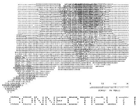
The Lab was formed in 1965 with a grant from the Ford Foundation to develop and sell a program called SYMAP, a computer mapping program that could produce overlay maps and output them on a line printer. The original goal of the Lab was to develop SYMAP as a software product, with the assumption that anyone with the hardware would also have a line printer. At the time, the concept of software as a product was revolutionary. Computer sales in the mid-1960s were primarily focused on hardware, and software was often included for free (Chrisman 2006, slide 3). Though the concept of software as a product was there, the Lab underestimated the complexity of making the concept a reality (Artz 2007).
The staff and students at the Lab lived and breathed mapping. They spent countless hours hunching over IBM keypunch machines creating the programs and data used to make the software and maps. The punch cards would then have to be brought to the nearby Harvard Computer Center where the decks would be turned over to the processor to run the batch (program and data). It was the only computer on campus, so during the day, turnaround time was typically eight hours. The staff and students at the Lab learned to visit the center at midnight when the turnaround was more like two hours. However, if their code contained errors, it was back to the keypunch machine in hopes of getting a map the next time.
SYMAP Connecticut Map (M. Friendly and D.J. Denis Early SYMAP image of Connecticut 2001)
The Lab also offered spatial analysis services and data creation as a way to generate additional revenue and stay afloat. One of the projects the Lab embarked on, the Urban Atlas Project, was with the USCB and the National Science Foundation to restructure urban atlas files. The project’s goal was to create atlases for each of the nation’s major metropolitan areas. This required digitizing maps for some 35,000 census tracts. This project revealed weaknesses in the Lab’s existing mapping program and, as a result, in the mid-1970s the Lab developed ODYSSEY, a vector-based GIS system, with Scott Morehouse as one of the core developers. With ODYSSEY’s ability to overlay maps very quickly, it eventually became the prototype for modern GIS (Artz 2007) (Coppock and Rhind 1991).
ODYSSEY was a big success for the Lab, but it also put the Lab in a difficult situation: how should Harvard handle the potential success of a commercial product? In 1981, the Lab had signed numerous contracts and over forty employees were preparing for the commercial debut of ODYSSEY. Ultimately, though, Harvard decided that the University should not be in the business of selling commercial products, which eventually led to the demise of the Lab. The private sector, however, saw this as an opportunity.
Environmental Systems Research Institute
The Environmental Systems Research Institute (ESRI) was established in 1969 and was one of a handful of GIS companies that spawned out of the Lab (others include Intergraph, ComputerVision, and Symercom, however, they all approached GIS from a CAD perspective) (ESRI “History of GIS”). But, it’s interesting to note how chance and timing played into this company’s huge success. You can trace ESRI back to the University of Minnesota, where ESRI’s founder, Jack Dangermond, was a student exploring digital mapping.
In an interview for the Youtube channel GIShistory, Jack discusses how the Lab had an impact on his work in the field of GIS. Jack describes how while he was at Minnesota, he discovered a small article about the Lab and decided he had to visit. He recalls that while at the Lab he met the Lab’s founder, Howard Fisher, who had a memorable and fanatical personally. Howard was impressed with Jack’s work and told Jack the whole history of the Lab in one afternoon (while Jack’s wife waited in the car) and then said, “You’ve just got to work here!” And so Jack did. Jack became a research assistant at the Lab from 1968 to 1969. (And as Jack says in the interview, he “was paid well,” receiving a [whopping] $4.40 an hour!) (“Jack Dangermond talks about the Harvard Laboratory for Computer Graphics and Spatial Analysis” 2009).
Jack recalls that in the early days, it was hard to make a digital map. One of his first computer maps took him about thirty submissions over the course of a month (“Allan Schmidt talks about the Harvard Laboratory for Computer Graphics and Spatial Analysis, Part 1” 2009). He created it using punch cards and a mainframe computer. Ultimately, Jack was able to help advance the field of GIS through his time at the Lab.
While Jack was there, Allan Schmidt (the executive director at the time) helped Jack launch the whole vision and idea of what became ESRI. ESRI began primarily as a nonprofit doing environmental consulting work. Then in the 1970s, ESRI developed a cell-based package called GRID and then a vector system called PIOS to perform analyses (ESRI “History Up Close,” 2015).
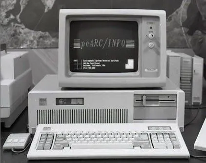
Initially, ESRI used the mainframe computer at the University of California to do all of the company’s processing. Eventually, ESRI purchased its own minicomputer and in 1982 it launched ARC/INFO, which is often called the first commercial GIS (ESRI “History Up Close” 2015). At that point, ESRI began advertising its product as a turnkey, do-it-yourself GIS. ESRI also shifted from a nonprofit to a for-profit organization. ESRI’s ability to make ARC/INFO work across computer platforms ranging from personal computers, workstations, minicomputers, and large mainframe computers was a huge factor in the product’s success.
ARC/INFO on PC in 1986 (ArcGIS 1986 PC ARC/INFO Released)
Another critical moment for the company was when Scott Morehouse, the development lead on the ODYSSEY project, left the Harvard Lab in 1981 to join ESRI. He brought with him the framework that eventually grew into ESRI’s next generation of GIS. ESRI called it ArcInfo and it is often considered the first modern GIS (“History Up Close” 2015).
Since the early 1970s, ESRI has expanded from a nonprofit with a staff of 15 to a global company of well over 3,800 employees.
The Early Days at ESRI (ArcGIS 1986 PC ARC/INFO Released)

The Development of National Datasets
Software advancements were certainly a large piece of the digital-mapping puzzle, but without readily available data, progress in this arena would have been slowed. Fortunately, a few agencies within the US federal government had vested interest and made headway. Two of the front-runners were the USCB and the USGS, and their timing was fitting.
US Census Bureau
Since its inception, the USCB has been tasked with storing and analyzing large datasets. (As you might recall, the USCB was the agency that helped advance the tabulating machine, which eventually morphed into IBM’s first database.)
One of the USCB’s challenges entering the 1960s was determining how to automate address matching. The USCB was required to produce area-based tabulations based on the postal address from returned mailing surveys. In the 1970s, the USCB developed a solution it called Dual Independent Map Encoding (USCB “Dual Independent Map Encoding” 2019). Essentially, this was an encoding system for describing geographic data. The DIME program used intersections, streets, and blocks, which are now analogous to points, lines, and polygons. The data was stored as map coordinates on punch cards. Computers would then create maps based on these punch cards.
The DIME project created a need for more data, and the data created for the project was stored as geographic base files (GBF/DIME). By the end of the 1970s, the USCB had created GBF/DIME files for every US city, which gave the Bureau a schematic street map within its tabulation areas. During the 1980s these files became key components to what eventually became the TIGER files (USCB “Dual Independent Map Encoding” 2019).
It’s difficult to overstate how important TIGER files were, not only to the 1990 census but also to the development of many local and regional datasets. These files provided a reliable base layer that many GIS offices used to further build out their in-house datasets. TIGER data was also one of the first glimpses of a seamless national dataset, and it currently makes up the base data for OpenStreetsMap.
USCB Logo for the United States Census Bureau’s TIGER (Topologically Integrated Geographic Encoding and Referencing) map data format
![]()
USGS
The USGS was on a similar track converting and generating digital map data.
Since 1879, the USGS has been entrusted with the responsibility of systematically mapping the nation (Rabbitt 1989). Under the direction of John Wesley Powell, the agency began creating the classic topographic maps in 1884 that we’re so familiar with (Usery, Varanka, and Finn n.d., 1).
These early maps began as hand sketches created by field surveyors and included features such as civil divisions, public works, hydrography, and hypsography, but by the 1930s the USGS started using aerial photography and photogrammetry.
Demand for maps with greater detail led to the production of the 1:24,000-scale, 7.5-minute quadrangle topographic maps. These are arguably the USGS’s most popular maps. Production of these maps began in the 1940s (USGS “National Geospatial Program”), and by 1991 they were declared complete (Usery, Varanka, and Finn n.d., 1). At that point, they were the most complete large-scale maps for the nation (Usery, Varanka, and Finn n.d., 1).
USGS 7.5 Minute Map (HowToWilderness.com Aerial Photo Stowe VT)

The USGS fully embraced the idea of digital mapping in the 1970s, though all of the Survey’s map data was in analog form (i.e., in paper form). USGS’s solution was to digitize the map features on the 7.5-minute maps and output digital cartographic binary files (USGS “Overview of the USGS Digital Raster Graphic [DRG] Program” 2017). This was the beginning of the DLGs that most of us GIS folks are so familiar with.
The USGS also developed a land-cover mapping program in the 1970s that generated land-use and land-cover information from remotely sensed imagery. Digital data was created for hydrologic units, political boundaries, census tracts, and federal lands. Under the program, the USGS developed a GIS (specifically the GIRAS) to tabulate the land cover by county or hydrologic unit. As a result of this program, digital map data was generated for the entire United States in an arc-node vector format (Coppock and Rhind 1991, 31).
In 1987, the USGS developed the concept for the creation of DOQs. Essentially, these are computer-generated images from aerial photographs in which displacement, caused by camera tilt or terrain relief, is removed. We are now accustomed to seeing this as aerial imagery in GIS, but this was a significant advancement at the time. The DOQs became a standard base layer for control (Usery, Varanka, and Finn n.d., 6).
The USGS began scanning its popular 7.5-minute maps in 1995 (USGS “Overview of the USGS Digital Raster Graphic [DRG] Program” 2017). These TIFFs became known as DRGs and were georeferenced to the UTM coordinate system. The DRGs were very useful as digital base map layers or for digitizing the approximation of known features.
Other notable USGS GIS data contributions include the NED and the NHD.
A significant factor in the success of digital mapping can be contributed to the decision by the USGS to make all map datasets freely available online and in the public domain. This allowed the software industry to focus on software with the notion that end users would have access to readily available, high-quality data.
Access to seamless, nationwide GIS data got even easier in 2001 when the USGS debuted The National Map (Usery, Varanka, and Finn n.d., 10) (also see The National Map, USGS). As a collaborative effort with other federal, state, and local partners, data was made available in a central location. Data can be downloaded from the map through an interactive application, and map layers include transportation, structures, orthoimagery, hydrography, land cover, geographic names, boundaries, and elevation. This concept laid much of the groundwork for many commercial products that subsequently sprung up, such as MapQuest and Google Maps.
The USCB and the USGS have both played invaluable roles in advancing GIS. Not only did they provide free, seamless national datasets, they also helped advance vector-based GIS and the topological model.
Overlaying the Stories
The motivation for GIS has varied widely, but most of the field’s innovation grew from academic curiosity and the governmental challenges of looking for solutions with large datasets (Coppock and Rhind 1991, 21–43).
When you explore the individual stories of GIS history, you see that chance, timing, and heritage played into its development.
You see how the British, with their obsession with surveying and mapping, laid much of the groundwork for GIS and that many of the early key players in mapping were of British heritage. Not only did they have access to accurate maps and tools — they were also wired with the mindset that mapping advances society.
Yet, it took the composition of North America to give rise to the first GIS. The abundance of public land in Canada and the United States (which Britain lacked) created the need for complex land management systems. You see that by the early 1980s, there were more than one thousand GIS systems in North America alone, which, proportionately, was extremely high (Tomlinson 1985).
But development of the first GIS also took a bit of chance. It wasn’t enough for the British-born Roger Tomlinson to have conceived the concept; it also took him sitting in the right seat on the right plane (i.e., next to Lee Pratt) on the right day to close the final gap.
The first generation of GIS was dominated by mainframe computers and punch card technology. You see the recurrence of the IBM System 360 in the 1960s and its ability to be programmed to cover a range of applications.
You also see how timing played a role in the second generation of GIS, as personal computing and software applications were the focus. Jack Dangermond’s timing at the Lab put him in position to successfully launch ESRI, and then, by the 1980s, personal computers were prevalent enough for ESRI to bring the first cross-platform, do-it-yourself GIS application to market.
The current GIS platform is built on web applications, shareable web services, and cloud computing. But, in this article we explored the interwoven stories that you discover when you zoom in on the history of GIS. Hopefully, when you zoom back out you will now have a greater appreciation for today’s GIS.

Note: a special thanks to the editor, Anna Tribolet for her awesome editing skills and for the creation of the ‘Key Moments in GiS’ infographic!
Sources
-
Aguirre, Jessica Camille. “The Unlikely History of the Origins of Modern Maps.” Smithsonian.com. June 2, 2014. Accessed August 19, 2019. https://www.smithsonianmag.com/history/unlikely-history-origins-modern-maps-180951617/, opens in a new tab.
-
Anam, Aysha. “How India was measured: Story of the Great Trigonometrical Survey of India.” India Today. Published July 10, 2018. Updated July 12, 2018. Accessed August 19, 2019. https://www.indiatoday.in/education-today/gk-current-affairs/story/how-was-india-measured-why-is-it-important-to-measure-land-1281835-2018-07-10, opens in a new tab.
-
ArcGIS. 1986 PC ARC/INFO Released. Retrieved from “Our Common History” story map. https://www.arcgis.com/apps/MapJournal/index.html?appid=df8224427fc741ab9f8117e9af1d692a, opens in a new tab.
-
Artz, Matt. “Charting the Unknown: How Computer Mapping at Harvard Became GIS.” GIS and Science. November 17, 2009. Accessed August 19, 2019. https://gisandscience.com/2009/11/17/charting-the-unknown-how-computer-mapping-at-harvard-became-gis/, opens in a new tab.
-
Beniger, James Ralph. The Control Revolution: Technological and Economic Origins of the Information Society, 411–412. Cambridge (MA): Harvard University Press, 1997. Accessed on 7/31/2019 via Google Books.
-
Chrisman, Nicholas. “Remembering the Lab: A short history of GIS at Harvard.” Presentation. 2006. Accessed August 19, 2019. https://docplayer.net/12667857-Remembering-the-lab.html, opens in a new tab.
-
Chrisman, Nick. Charting the Unknown: How Computer Mapping at Harvard Became GIS. Redlands, CA: Esri Press, 2006.
-
Coppock, J. Terry, and David W. Rhind. “The History of GIS.” In Applications. Vol. 2 of Geographical Information Systems: Principles and Applications. Edited by David J. Maguire,
-
Michael F. Goodchild, and David W. Rhind, 21–43. Harlow, UK: Longmans, 1991. https://oxfordbibliographiesonline.com/view/document/obo-9780199874002/obo-9780199874002-0143.xml#obo-9780199874002-0143-bibItemGroup-0001, opens in a new tab.
-
DeMers, Michael. “CGIS History Captioned.” Youtube. Uploaded by Michael DeMers on August 29, 2013. Accessed August 19, 2019. https://www.youtube.com/watch?v=3VLGvWEuZxI, opens in a new tab.
-
DeMers, Michael. CGIS Screenshot. 2013. Screenshot from “CGIS History Captioned” YouTube video. https://www.youtube.com/watch?v=3VLGvWEuZxI, opens in a new tab.
-
ESRI. “History of GIS.” Accessed August 19, 2019. https://www.esri.com/en-us/what-is-gis/history-of-gis, opens in a new tab.
-
ESRI. “History Up Close.” 2015. Accessed August 19, 2019. https://www.esri.com/~/media/Files/Pdfs/about-esri/esri-history-up-close, opens in a new tab.
-
Fisk, Dale. “Programming with Punched Cards.” Columbia University. Accessed August 19, 2019. https://www.columbia.edu/cu/computinghistory/fisk.pdf, opens in a new tab.
-
Friendly, M. & Denis, D. J. Early SYMAP image of Connecticut. 2001. “1950-1974: Re-birth of data visualization” article on Milestones in the history of thematic cartography, statistical graphics, and data visualization site. https://www.datavis.ca/milestones/, opens in a new tab. Accessed August 29, 2019.
-
Garfield, Simon. On the Map: A Mind-Expanding Exploration of the Way the World Looks, 192, 194. New York: Gotham Books, 2013.
-
GIS Geography. “The Remarkable History of GIS.” June 13, 2019. Accessed August 19, 2019. https://gisgeography.com/history-of-gis/, opens in a new tab.
-
GIS Geography. “USGS Formats DLG, DRG and DOQ – Vector and Raster Formats.” Last updated January 5, 2019. Accessed August 19, 2019. https://gisgeography.com/usgs-formats-dlg-drg-doq/, opens in a new tab.
-
GIS Geography.“TIGER GIS Data (Topologically Integrated Geographic Encoding & Referencing).” Last updated April 25, 2019. Accessed August 19, 2019. https://gisgeography.com/tiger-gis-data-topologically-integrated-geographic-encoding-referencing/, opens in a new tab.
-
GISHistory. “Allan Schmidt talks about the Harvard Laboratory for Computer Graphics and Spatial Analysis, Part 1.” Youtube. Uploaded on November 2, 2009. Accessed August 19, 2019. https://www.youtube.com/watch?v=B14LfcJN490&feature=youtu.be, opens in a new tab.
-
GISHistory. “Jack Dangermond talks about the Harvard Laboratory for Computer Graphics and Spatial Analysis.” Youtube. Uploaded on October 30, 2009. Accessed August 19, 2019. https://www.youtube.com/watch?v=BaHXDMid78I&feature=youtu.be, opens in a new tab.
-
HowToWilderness.com. Aerial Photo Stowe VT. Retrieved from “Reading a Map” article. https://howtowilderness.com/map-training/, opens in a new tab.
-
Jones, Douglas W. “Punched Cards: A brief illustrated technical history.” The University of Iowa Department of Computer Science. Last modified June 28, 2017. Accessed August 19, 2019. https://homepage.divms.uiowa.edu/~jones/cards/history.html, opens in a new tab.
-
Library of Congress. Image of punched card of Herman Hollerith. 1895. Retrieved from Wikipedia Commons image “File:Hollerith Punched Card.jpg.” https://memory.loc.gov/mss/mcc/023/0008.jpg, opens in a new tab.
-
Micronautes. Broad Street Map/Broadwick Street Water Pump. 2017. Retrieved from “John Snow and cholera” article by Laura Gómez. https://unautes.com/index.php/2017/11/16/john-snow-and-cholera/?lang=en, opens in a new tab.
-
Ordnance Survey. “Our History.” 2019. Accessed August 19, 2019. https://www.ordnancesurvey.co.uk/about/overview/history.html, opens in a new tab.
-
Parecki, Aaron. Esri in 1969. Jack Dangermond, Scott Morehouse, SJ Camarata, Logan Hardison. 2013. Retrieved from Flickr. https://www.flickr.com/photos/aaronpk/9570322487/in/photostream/, opens in a new tab.
-
Pascual, Daniel Fernández. Great Trigonometrical Survey of India. 2012. Retrieved from “Mapping an Empire” article on Deconcrete.org. https://www.deconcrete.org/2012/03/12/mapping-an-empire/, opens in a new tab.
-
Poiker, Thomas K., and Ian K. Crain. “Geographic Information Systems.” In The Canadian Encyclopedia. Historica Canada. Article published February 07, 2006; Last edited February 3, 2014. Accessed August 19, 2019. https://www.thecanadianencyclopedia.ca/en/article/geographic-information-systems, opens in a new tab
-
Rabbitt, Mary C. “The United States Geological Survey: 1879-1989.” Circular, 1989. https://pubs.usgs.gov/circ/1050/pdf/CIRC1050.pdf, opens in a new tab.
-
Schuster, Adam. Proto IBM. 2007. Retrieved from Flickr. https://www.flickr.com/photos/44124384537@N01/411109339, opens in a new tab.
-
Thompson, Clive. “From Ptolemy to GPS, the Brief History of Maps.” Smithsonian Magazine. July 2017. Accessed August 19, 2019. https://www.smithsonianmag.com/innovation/brief-history-maps-180963685/, opens in a new tab.
-
Tomlinson 1984: Geographic Information Systems - the new frontier. The Operational Geographer 5: 31-6.
-
Tomlinson, Roger. “Origins of the Canada Geographic Information System.” ESRI. 2012. Accessed August 19, 2019. https://www.esri.com/news/arcnews/fall12articles/origins-of-the-canada-geographic-information-system.html, opens in a new tab.
-
University Consortium for Geographic Information Science. “Roger Tomlinson.” Accessed August 19, 2019. https://www.ucgis.org/roger-tomlinson, opens in a new tab.
-
US Census Bureau.“Agency History.” Last revised May 30, 2019. Accessed August 19, 2019. https://www.census.gov/history/www/census_then_now/, opens in a new tab.
-
US Census Bureau. “Census Bulletin.” Published September 6, 1968. Accessed August 19, 2019. https://www.census.gov/history/pdf/1968censusbulletin-dime.pdf, opens in a new tab.
-
US Census Bureau. “Dual Independent Map Encoding.” Last revised May 30, 2019. Accessed August 19, 2019. https://www.census.gov/history/www/innovations/technology/dual_independent_map_encoding.html, opens in a new tab.
-
US Census Bureau. “Herman Hollerith.” Last revised May 17, 2018. Accessed August 19, 2019. https://www.census.gov/history/www/census_then_now/notable_alumni/herman_hollerith.html, opens in a new tab.
-
US Census Bureau. Logo for the United States Census Bureau’s TIGER (Topologically Integrated Geographic Encoding and Referencing. Retrieved from Wikipedia Commons image “File:US-Census-TIGERLogo.svg.” https://commons.wikimedia.org/wiki/File:US-Census-TIGERLogo.svg, opens in a new tab.
-
US Geological Survey. “3D Elevation Program (3DEP).” Accessed August 19, 2019. https://www.usgs.gov/core-science-systems/ngp/3dep/about-3dep-products-services, opens in a new tab.
-
US Geological Survey. “National Geospatial Program.” Accessed August 29, 2019. https://www.usgs.gov/core-science-systems/national-geospatial-program/topographic-maps, opens in a new tab.
-
US Geological Survey. “Overview of the USGS Digital Raster Graphic (DRG) Program.” Last modified May 11, 2017. Archived February 9, 2018. Accessed August 19, 2019. https://archive.usgs.gov/archive/sites/topomaps.usgs.gov/drg/drg_overview.html, opens in a new tab.
-
US Geological Survey. The National Map. Last modified October 22, 2018. https://viewer.nationalmap.gov/advanced-viewer/, opens in a new tab.
-
Usery, E. Lynn, Dalia Varanka, and Michael P. Finn. “Mapping Developments and GIS in the USGS, 1884-2009.” International Cartographic Association. Accessed August 19, 2019. https://icaci.org/files/documents/ICC_proceedings/ICC2009/html/nonref/7_13.pdf, opens in a new tab.
-
Waldheim, Charles. “The Invention of GIS.” The Harvard Gazette. Video/Production: Ned Brown. October 12, 2011. Accessed August 19, 2019. https://news.harvard.edu/gazette/story/2011/10/the-invention-of-gis/, opens in a new tab.
-
Winfields Outdoors. Image 1 from “Interview With Ordnance Survey - History & Future of OS Maps” article. February 18, 2016. Accessed August 29, 2019. https://www.winfieldsoutdoors.co.uk/blog/ordnance-survey-interview/, opens in a new tab.
_[3DEP]: 3D Elevation Project _[CAD]: Computer-aided design _[DEM]: Digital elevation model _[DLG]: Digital line graphs _[DOQ]: Digital Orthophoto Quadrangle _[DRG]: Digital raster graphics _[GIRAS]: Geographic Information Retrieval and Analysis System _[NED]: The National Elevation Dataset provided seamless, high-resolution raster elevation data for the entire nation in the form of DEM layers. This project was replaced by the 3DEP. (“3D Elevation Program [3DEP],” USGS). _[NHD]: The National Hydrography Dataset is a comprehensive GIS dataset consisting of surface water in the United States, including lakes, ponds, streams, rivers, canals, and oceans. _[PIOS]: Planning Information Overlay System _[TIGER]: Topologically integrated geographic encoding and referencing _[USCB]: US Census Bureau _[USGS]: US Geological Survey _[UTM]: Universal Transverse Mercator