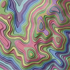
While technology advances towards products with greater resolution and accuracy, sometimes more data isn’t always better data. Sometimes, being able to see general trends and relative differences paints a more interesting picture than sub foot imagery oLidar . This is the case when terrain is dumbed down and represented with generalized contour polygons.
 Generalized contour polygons are relatively easy to create (no GISP required) and allows the user multiple ways to symbolize the data depending on the desired cartographic effect. Probably the most difficult part of creating the contours is deciding how much to generalize the terrain and what contour interval is best suited for the intended scale, unfortunately a bit of trial and error can be involved. An added benefit of creating contour polygons are the derivative data products like Tanaka contours that can be created once the base elevation and polygons are generated.
To create contours using the steps below you will need a DEM and ArcGIS with the Spatial Analyst Extension.
Step 1
Get your units straight. If you want your contours in feet and your DEM is meters (it probably is), now is the time to fix that with a little raster math, opens in a new tab.
arcpy.Times_3d(r'C:\Contours.gdb\dem30', 3.28084, r'C:\Contours.gdb\dem30_feet')Step 2
Start generalizing… This step can involve a bit of trial and error but is worthwhile spending the time to get it right since all your data will be created from this output. To generalize or smooth a DEM use focal statistics, opens in a new tab. This tool will calculate a new value for each cell in the DEM based on the neighboring cells around it and the statistical method defined. The larger the neighborhood specified, the more the DEM will be smoothed or generalized.
arcpy.CheckOutExtension('spatial')
from arcpy.sa import *
outDEM = FocalStatistics(r'C:\Contours.gdb\dem30_feet', NbrCircle('25', 'CELL'), 'MEAN')
outDEM.save(r'C:\Contours.gdb\dem30_foc25')
Step 3
Figure out the contour interval and reclassify your DEM. To start, you will want to know the minimum and maximum values of your DEM. The easiest way to do this is right click the DEM in ArcCatalog and find the values under Statistics in the Raster Dataset Properties. Once you know the minimum/maximum values of your DEM you can define your contour interval and set up the code to reclassify your DEM.
When reclassifying, opens in a new tab the DEM, you will be assigning elevation ranges defined by your contour interval to a new value. For example, if the minimum value of your DEM is 3000 feet and your contour interval is 200 ft, all elevations from 3000 to 3200 will be calculated to a new elevation of 3200. This will be done for all elevations in your DEM based on the contour interval, basically creating a DEM of terraces. Setting up the code for this part takes a little time, especially if your contour interval is small and your min/max elevation range is large, but on the plus side, you only have to do it once. Your code will look something like this:
import arcpy
from arcpy import env
from arcpy.sa import *


arcpy.CheckOutExtension('spatial')
env.workspace = r'C:\Contours.gdb'
#Define ranges for entire DEM
newRange = RemapRange([[3000, 3200, 3200], [3200.1, 3400, 3400], [3400.1, 3600, 3600], [3600.1, 3800, 3800], \
                       [4600.1, 4800, 4800] ,,,,,,,,,,,,,,, [13200.1, 13400, 13400], [13400.1, 13600, 13600]])
outRaster = Reclassify('dem30_foc25', 'Value', newRange)
outRaster.save('dem30_reclass')
Step 4
Convert your reclassified raster to polygons, opens in a new tab. Your elevation raster is set up, you’re almost done.
arcpy.RasterToPolygon_conversion(r'C:\Contours.gdb\dem30_reclass', 'ContourPolygons', 'SIMPLIFY', 'VALUE')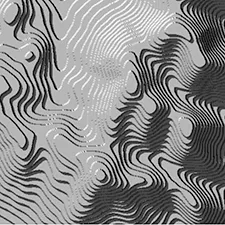 If you’ve made it this far and created contour polygons, you might as well and take it a step further and create Tanaka contours, opens in a new tab. Tanaka contours were developed by Japanese cartographer Tanaka Kitiro in 1950. Using this technique terrain is represented by a terraced effect with the leading northwest edge of the contour illuminated by a light source and the opposite side in shadow.
To create Tanaka contours all you need is your reclassified DEM. To start, create 2 hillshades, opens in a new tab, one with shadows and another without.
arcpy.HillShade_3d(r'C:\Contours.gdb\dem30_reclass', 'ContourHillshd_shad', '#', '#', 'SHADOWS')
arcpy.HillShade_3d(r'C:\Contours.gdb\dem30_reclass', 'ContourHillshd_noshad', '#', '#', 'NO_SHADOWS')
And finally, highlight the illuminated edges and shadows with an aspect raster, opens in a new tab.
arcpy.Aspect_3d(r'C:\Contours.gdb\dem30_reclass', 'ContourAspect') Now that you’ve spent all this time creating data, it’s time to start experimenting with how it’s symbolized in ArcMap. For the two hillshades all you’ll need to do is adjust the transparency to your liking. For the aspect layer you will need to open the
 Layer Properties Symbology tab and check the box next to Display Background Value and set the value to -1 and the color to transparent. This will remove all the black areas, leaving the portions of the contours that are either illuminated or shadowed. Everything else is a matter of personal preference.
If you had trouble creating any of the layers in the steps above, or are interested in layer files for symbology, everything can be downloaded, opens in a new tab.
If you have a favorite cartographic technique or dataset that you would like to highlight, please send it our way.