Python Shorts: Point Me to the Nearest Points with GeoPandas

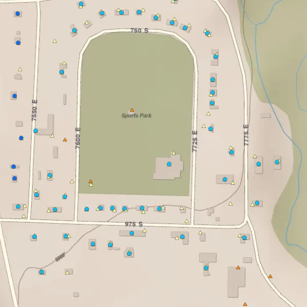
One analysis that comes up regularly in GIS is figuring out the relationship between two different sets of data. For example, let’s say we’ve got an address point layer (symbolized with circles) and a table of temperature readings identified by latitude and longitudes (symbolized with triangles), and we want to know the address of each temperature point.

Near(ly) There

Because we’re GIS people and think spatially, our first instinct is to run a Near analysis to find the features from the address point layer that are closest to each temperature feature. This creates a key we can use to join the second layer to the first.

If we’re lucky, there’s a one-to-one relationship where each address is only the closest point for one temperature reading. The next step is to choose a distance threshold to eliminate any obviously wrong associations—but how can we manually review our distance threshold to make sure it’s right? How do we know which temperature readings are associated with which address point when we plot them out on a map?

And then there’s the case when we get a one-to-many relationship: multiple temperature readings that all claim a single address point as their closest point. How do we know which point to choose? Is the nearest always right? How do we review that?

A Helpful Pointer

A line pointing from each temperature reading to its associated address point would make comparing the points visually a breeze. However, there’s not an intuitive way to create this using the normal near analysis tools.

GeoPandas gives us an easy way to both create the near table for joining the two layers and then creating this new line layer that points between the two layers. This lets us see these associations without having to refer to identifiers in the attribute tables or cluttering our map with labels.

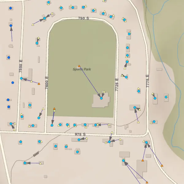
These lines, symbolized with an arrow at the ends, help us see where multiple temperature data points (triangles) are associated with single address points (circles). We can also see temperature points that are offset from address points and determine if that’s an artifact of slight offsets in data collection locations or if there’s not an address nearby so it’s grabbing the neighboring point instead.

Step zero: Prep the data

Before we can create the lines, we need to make sure the layers are both in the same projected CRS. We can use gpd.GeoDataFrame.to_crs, opens in a new tab to reproject our layers.

Step one: Perform the near analysis

Use gpd.sjoin_nearest, opens in a new tab to assign the points from the second layer to the closest point in the first layer.

nearest = gpd.sjoin_nearest(
    temperature_layer,
    address_point_layer,
    how="left",
    distance_col="distance_m",
    lsuffix="_temps",
    rsuffix="_addresses")

This gives us a dataframe with a row for each feature in the temperatures layer, including their geometries. It joins the columns from the nearest address point to these rows, including an index__addresses column that we can use to join the resulting dataframe back to the address dataframe. Alternatively, we could use a unique key in our address points layer to perform the join. The distance_col argument specifies a column to hold the distance between the temperature record and its associated address point.

Step two: Merge the resulting table back to the address points to get their geometries

The gpd.sjoin_nearest operation only returns the geometries from one of the input dataframes, so we need access to the other. Because GeoPandas can handle multiple geometry columns, we’ll use the index__addresses column to create a new dataframe with both temperature and address point geometries for each row in our output dataframe.

both_points = nearest[["index__addresses", "distance_m", "geometry"]].merge(
    address_points[["address", "city", "state", "zip", "geometry"]],
    how="left",
    left_on="index__addresses",
    right_index=True,
    suffixes=("_temperature", "_address"))

The resulting dataframe will now have two geometry columns named geometry_temperature and geometry_address (thanks to the suffixes argument).

Step three: Create a new linestring geometry between the two points

Now that we have the geometries for the temperature and address point for each row, we can use them as the start and end points for a new linestring geometry.

from shapely.geometry import LineString

both_points["geometry"] = both_points.apply(
    lambda row: LineString([row["geometry_temperature"], row["geometry_address"]]),
    axis=1)

Step four: Write the new linestring features to disk

The final step is to write the linestring features to disk as a new layer. To do this, we’ll set the new line as the geometry column and drop the columns with the original point geometries.

both_points.set_geometry("geometry", crs="EPSG:26912") \
           .drop(columns=["geometry_temperature", "geometry_address"]) \
           .to_file(
                r"C:\path\to\output.gdb",
                layer="temperatures_to_address_points",
                engine="pyogrio",
                driver="OpenFileGDB")

Now we can add the line layer to a map, add arrows onto the end, and get a nice visual representation of which temperature readings are associated with which address points.

The beauty of GeoPandas is that we can do this in a couple of lines of code without having to write any intermediate datasets to disk. This keeps our geodatabases uncluttered and documents our process for future reference and repeatability.