
I recently discovered Uber’s open-source H3 geospatial indexing system, opens in a new tab while working on a project with a lot of point data. This is a great tool for aggregating points into regularly-sized polygon geometries so that you can map and evaluate the spatial trends of a point-based phenomenon, but it needs a bit of an introduction to understand why it’s great and how to use it with traditional GIS data.
The Status Quo: Slow and Incompatible
You’ve probably aggregated and mapped point data before by using the Summarize Within tool to spatially join your points to other boundary datasets, like cities or counties. Census tracts or blocks are often popular targets, allowing you to compare your data to census data.
However, administrative boundaries like tracts, cities, or political districts are inherently irregular. They don’t “tile the plane” in a standard, repeating pattern that allows you to see how a dataset changes over space.
Because hexagons are the bestagons, opens in a new tab, you may have created hex grids that cover their area of interest and then aggregate their point data to these hexes.
However, these custom hex grids are usually project-specific and don’t conform to any sort of common, well-known grid, making it difficult to pull in other hexed data. And while hexagons tile a plane beautifully, you can’t tesselate them to create a perfect larger hexagon, which means it’s difficult to create a larger or smaller grid that relates to your original grid. And as anyone who’s tried to aggregate a ton of points into a ton of hexagons can tell you, spatial joins can be slow.
H3 Uses Math, Not Spatial Operations
To understand how H3 solves these problems, we need to understand how it works. Coming from the GIS world, we think of the “point in polygon” problem spatially: search to see if the given point is inside the given area. We can then aggregate or summarize all the data within that area to come up with a single number or metric. However, with H3 we need to shift our thinking. H3 takes a lat/long and assigns an ID that corresponds to a mathematically-defined hex. There’s nothing inherently spatial about it, it’s all just math. The output is just a number.
It’s a Common Grid (kind of)
As an open-source system, H3 has become a sort of de facto standard. Anyone can use it, and anyone can take someone else’s data with H3 grid ids and compare it with their own. While it’s been around for a few years, there could be a novelty factor driving it’s adoption, so it remains to be seen how widely it will be adopted.
However, even if it doesn’t become the overwhelming global standard, the H3 system can still be useful for standardizing analyses across projects within an organization. If we at UGRC do a project for one state agency with the grid, it would be easy to pull that data into another project in the future knowing that they both use the same hexes.
H3 Handles Different Grid Resolutions Elegantly
It is mathematically impossible1 to create a larger hexagon from smaller hexagons, which means we can’t create a geographical hierarchy of hexes where one level of hexes perfectly cover the same area as a single larger hex. However, H3 makes a logical hierarchy by rotating the larger, parent hex to cover as much of its seven children as possible, as visible in the image below. The H3 indexing page, opens in a new tab has more detail on how this works.
The important point is that an individual hex ID contains the IDs of the hexes “above” it in the hierarchy, kind of like how census GeoIDs contain the block, tract, county, and state codes. This makes it easy to traverse up to a larger hex without re-calculating the IDs.
Using these multiple scales (which H3 calls resolutions), we can create hexes at multiple scales to aggregate our data to larger and larger areas. With these, we can view trends at the neighborhood, city, or county level. We can also create web maps that allow us to drill down from general trends to neighborhood or block level to see what areas contribute the most.
Assigning H3 IDs is Fast
As noted above, H3 uses some fancy mathematics under the hood to assign hex ids instead of doing spatial analysis. Written in C and exposed through a variety of bindings in other languages, these calculations are pretty darn fast at figuring out what hex cell a point belongs in.
For example, I used %timeit to assign a resolution 9 ID to all 1,339,635 of our address points (after projecting them to WGS84 to get direct access to lat/long in the SHAPE field):
def assign_h3(df, resolution):
    df[f'h3_{resolution}'] = df.apply(lambda row: h3.h3_to_string(h3.geo_to_h3(row['SHAPE']['y'], row['SHAPE']['x'], resolution)), axis=1)

addr_df = pd.DataFrame.spatial.from_featureclass(r'H3\H3.gdb\address_points_20220727_wgs84')

%timeit assign_h3(addr_df, 9)
> 23.8 s ± 377 ms per loop (mean ± std. dev. of 7 runs, 1 loop each)
24 Seconds for 1.3 million points. That’s fast 🏃♀️💨
Note: To get this speed, you’ll need to use the h3.api.numpy_int API as noted in the h3-py documentation, opens in a new tab
Using H3 Hexes in A Map: Analyzing Supermarket Availability
Ok, so we can assign a hex id to point data quickly and easily. But, at some point, we need a spatial representation of the hexes if we’re going to map out our summarized or aggregated data. Once we’ve got that, we can then use pandas to aggregate our data and join it to the hex geometries.
To show this in action, we’ll use our Open Source Places and the address points we investigated earlier to do a quick analysis of the number of addresses per grocery store throughout the state.
Creating an H3 Hex Feature Class
First, we need the actual polygons of the hexes themselves. The H3 API provides the polyfill method for identifying all hex IDs whose centroids are within a polygon along with the h3_to_geo_boundary method for returning the polygon corresponding to a specific hex ID.
In the code below we first buffer the state boundary so that we get all the hexes that cover the state. Then, we get the hex ids, get the polygons associated with those ids as geojson, and convert the geojson to a spatially-enabled dataframe. Finally, we write that dataframe out to disk.
state_boundary_df = pd.DataFrame.spatial.from_featureclass(r'H3\opensgid.ugrc.utah.gov.sde\opensgid.boundaries.state_boundary')

#: Buffer the state boundary by 5km
#: Row index 0 is a mask outside the state boundary, index 1 is the boundary itself.
#: Also, the SHAPE field is the last item in the column index
buffered = state_boundary_df.iloc[1, -1].buffer(5000)
buffered_df = pd.DataFrame.spatial.from_df(
                pd.DataFrame({'SHAPE': [buffered]}),
                geometry_column='SHAPE', sr=26912
                )

#: Project our polygon to WGS84 and convert to geojson for the H3 analysis
buffered_df.spatial.project(4326)
geojson_dict = json.loads(buffered_df.spatial.to_featureset().to_geojson)

#: Get both the hexagon numbers and their hexadecimal representation in string form
#: We have to specify the geometry from the first feature in the geosjon dict, even though we only have
#: one feature in there
resolution = 6
hexes = h3.polyfill(geojson_dict['features'][0]['geometry'], resolution, geo_json_conformant=True)
str_hexes = [h3.h3_to_string(h) for h in hexes]

#: Create a new spatially-enabled data frame by calling h3_to_geo_boundary and creating a Geometry object
#: in one fell swoop
#: And yes, it's generally bad form to assign a lambda function a name, but this helps break the code up
polygoniser = lambda hex_id: arcgis.geometry.Geometry({
                'rings': [h3.h3_to_geo_boundary(hex_id, geo_json=True)],
                'spatialReference': {'wkid': 4326}
                })
hexes_df = pd.DataFrame.spatial.from_df(
                pd.DataFrame({'hex_id': str_hexes, 'SHAPE': list(map(polygoniser, hexes))}),
                geometry_column='SHAPE', sr=4326
                )

#: Finally, write it out
hexes_df.spatial.to_featureclass(r'H3\H3.gdb\state_h3_6_wgs')
If geopandas and geojson is your thing, Guilherme M. Iablonovski has a write-up, opens in a new tab on Medium for this same process without any Esri formats or libraries. My code above is a translation of his process into Esri-land.
Aggregating Our Data per Hex and Joining the Polygons
Now that we’ve got the boundaries, we can do our analysis and map it out. First, we’ll use pandas’ groupby, opens in a new tab functionality on both the address points and open source places to group according to the hex id and get the count of unique records within each group. We then combine the two resulting series with the hex polygons, and finally we map the resulting data.
#: Load the open source places, project to lat/long, and get hex ids at level 6
osp_points_df = pd.DataFrame.spatial.from_featureclass(r'H3\opensgid.ugrc.utah.gov.sde\opensgid.society.open_source_places')
osp_points_df.spatial.project(4326)
assign_h3(osp_points_df, 6)
#: Perform the aggregation for each dataset and call the count() method on a column to get the number of features
#: in each group.
#: Note that we pre-filter the places to the 'supermarket' category.
addrs_per_hex = addr_df.groupby('h3_6')['utaddptid'].count()
supermarkets_per_hex = osp_points_df[osp_points_df['category']=='supermarket'].groupby('h3_6')['osm_id'].count()
#: Merge our two resulting series together into a dataframe, moving the hex id out of the index and renaming columns.
#: We also use dropna to drop any hexes that are missing either address points or supermarkets.
data_hexes = pd.concat([addrs_per_hex, supermarkets_per_hex], axis=1)
.dropna()
.reset_index()
.rename(columns={'utaddptid': 'addrs', 'osm_id': 'supermarkets'})
#: Calculate our new metric
data_hexes['addrs_per_supermarket'] = data_hexes['addrs'] / data_hexes['supermarkets']
#: Join our new data with the hex polygons, keeping only the ones
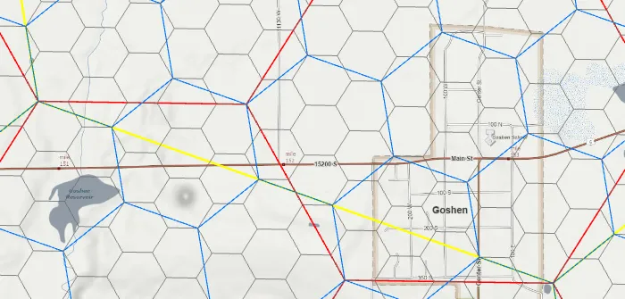
merged_df = hexes_df.merge(data_hexes, left_on='hex_id', right_on='h3_6', how='inner').sort_values(by='addrs_per_supermarket')At this point we can write the result out to disk or do whatever else we want with it. I went ahead and plotted it in a jupyter notebook to get the screenshot at the top of the page:
map1 = merged_df.spatial.plot(renderer_type='c',
                              method='esriClassifyQuantile',
                              col='addrs_per_supermarket',
                              class_count=5,
                              cmap='RdYlGn_r',
                              alpha=.5)
map1.center = [40.6, -111.9]
map1.zoom = 9
map1.take_screenshot()
The H3 grid/id system makes it quick and easy2 to do this spatial assignment, aggregation, and comparison without needing to fuss around with spatial joins, ArcGIS table joins, or summary statistics. Best of all, because it’s in code it’s easily repeatable and can be stored in version control (ie, GitHub).
Footnotes
-
Consider a regular polygon (a polygon where all interior angles have the same measurement and all sides are equal, like a square). If you want to place two polygons next to each other so that their outer edges create a straight line, they must have interior angles that, when placed next to each other, add up to 180 degrees.
For example, place two squares next to each other. Their top edges create a straight line above both squares, and the sum of the two interior angles that are adjacent to each other is 180 degrees (90 + 90). Or, place three equilateral triangles next to each other so that their three points all touch. The three 60 degree interior angles all add up to 180 degrees, and you have a flat line on top.
A regular hexagon has interior angles of 120 degrees. No matter how you rotate them, there is no way to place two hexagons next to each other so that their two interior angles add up to 180. Ergo, there is no way to place two hexagons next to each other so that any of the resulting boundaries create a straight line.
Because of this inability to form a straight line when we tile (or tesselate) hexagons together, we cannot create a larger, regular polygon (hexagon or otherwise) from hexagons. ↩
-
Just so long as your definitions of quick and easy involve a snake and copious amounts of Monty Python references. ↩